HACD: Hierarchical Approximate Convex Decomposition

October 2, 2011, 3:16 am

≫ Next: HACD optimization

$

0

0

Check out V-HACD 2.0!

I discovered the convex decomposition problem two years ago thanks to a very instructive discussion I had with Stan Melax. At that time, we needed a convex decomposition tool for the game we were working on.  Stan pointed me to John Ratcliff's approximate convex decomposition (ACD) library. Inspired by John's work I developed the HACD algorithm, which was published in a scientific paper at ICIP 2009.

The code I developed back then was  heavily relaying on John's ACD library and Stan's convex-hull implementation (thanks John and Stan :)! ). My implementation was horribly slow and the code was unreadable. When Erwin Coumans contacted me six moths ago asking for an open source implementation of the algorithm, I had no choice than re-coding the method from scratch (i.e. my code was too ugly :) !) . One month later, I published the first version of the HACD library.  Since then, I have been improving it thanks to John's, Erwin's and a lot of other peoples' comments and help. John re-factored the HACD code in order to provide support for user-defined containers (cf. John's HACD). Thanks to Sujeon Kim and Erwin, the HACD library was recently integrated into Bullet.

In this post, I'll try to briefly describe the HACD algorithm and give more details about the implementation. I'll provide also an exhaustive description of the algorithm parameters and discuss how they should be chosen according to the input meshes specificities. By doing so, I hope more people would get interested in the library and would help me improving it.

Why do we need approximate convex decomposition?

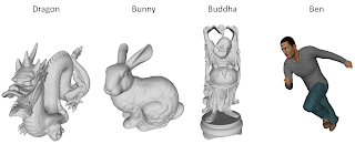
Collision detection is essential for realistic physical interactions in video games and computer animation. In order to ensure real-time interactivity with the player/user, video game and 3D modeling software developers usually approximate the 3D models composing the scene (e.g. animated characters, static objects...) by a set of simple convex shapes such as ellipsoids, capsules or convex-hulls. In practice, these simple shapes provide poor approximations for concave surfaces and generate false collision detections.

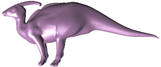
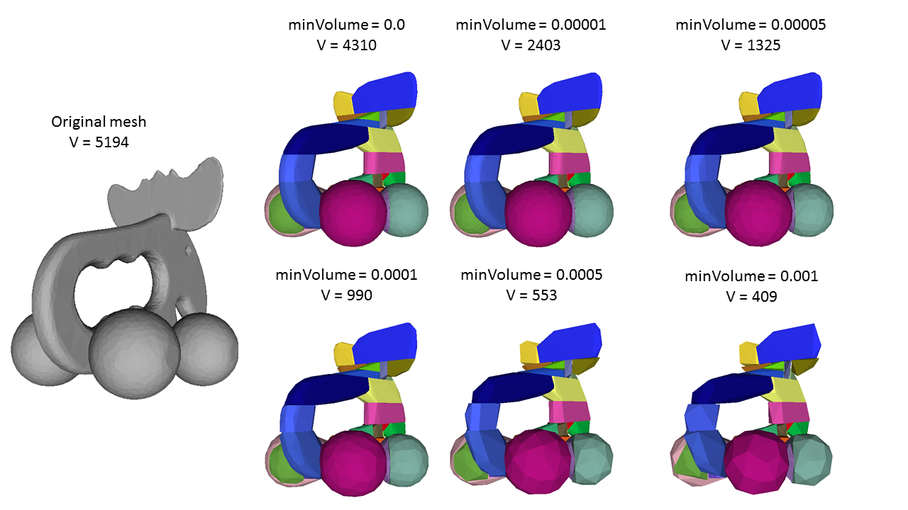
Original mesh

Convex-hull

Approximate convex decomposition

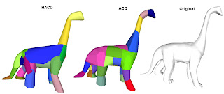
A second approach consists in computing an exact convex decomposition of a surface S, which consists in partitioning it into a minimal set of convex sub-surfaces. Exact convex decomposition algorithms are NP-hard and non-practical since they produce a high number of clusters. To overcome these limitations, the exact convexity constraint is relaxed and an approximate convex decomposition of S is instead computed. Here, the goal is to determine a partition of the mesh triangles with a minimal number of clusters, while ensuring that each cluster has a concavity lower than a user defined threshold.

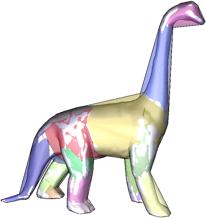
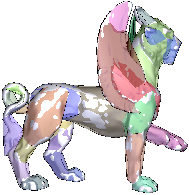
Exact Convex Decomposition produces 7611 clusters

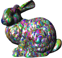
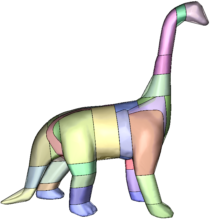
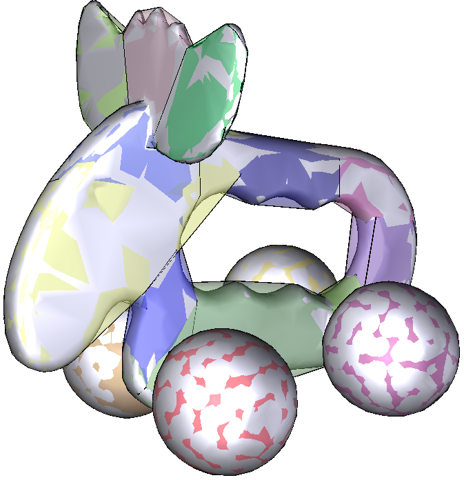
Approximate convex decomposition generates 11 clusters

What is a convex surface?
Definition 1: A set A in a real vector space is convex if any line segment connecting two of its points is contained in it.

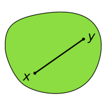
A convex set in IR2.

A non-convex set in IR2.

Let us note that with this definition a sphere (i.e. the two-dimensional spherical surface embedded in IR3)  is a non-convex set in IR3. However, a ball (i.e. three-dimensional shape consisting of a sphere and its interior) is a convex set of IR3.

When dealing with two dimensional surfaces embedded in IR3, the convexity property is re-defined as follows.


Definition 2: A closed surface S in IR3 is convex if the volume it defines is a convex set of IR3.

The definition 2 characterizes only closed surfaces. So, what about open surfaces?

Definition 3: An oriented surface S in IR3 is convex if there is a convex set A of IR3 such that S is exactly on the boundary of A and the normal of each point M of S points toward the exterior of A.


The definition 3 do not provide any indication of how to choose the convex set A. A possible choice is to consider the convex-hull of S (i.e. the minimal convex set of IR3 containing S), which lead us to this final definition.

Definition 4: An oriented surface S in IR3 is convex if it is exactly on the boundary of its convex-hull CH(S) and the normal of each point M of S points toward the exterior of CH(S).

With Definition 4, the surface defined by the half of a sphere is convex. The half of a torus is not convex.

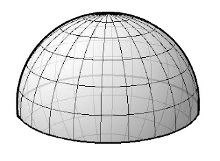
Half of a sphere is convex.

Half of a torus is not convex.

How to measure concavity?
There is no consensus in the literature on a quantitative concavity measure. In this work, we define the concavity C(S) of a 3D mesh S, as follows:

C(S) = argmax ∥M − P (M )∥, M∈S

where P(M) represents the projection of the point M on the convex-hull CH(S) of S, with respect to the half-ray with origin M and direction normal to the surface S at M.

Concavity measure for 3D meshes: distance between M0 and P(M0) (Remark:  S is a non-flat surface. It is represented in 2D to simplify the illustration)

Let us note that the concavity of a convex surface is zero. Intuitively, the more concave a surface the ”farther” it is from its convex-hull. The definition extends directly to open meshes once oriented normals are provided for each vertex.


In the case of a flat mesh (i.e., 2D shape), concavity is measured by computing the square root of the area difference between the convex-hull and the surface:

C_flat(S) = sqrt(Area(CH)-Area(S)).

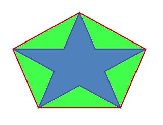
Concavity measure for closed 2D surfaces: the square root of the green area.

Here again, the concavity is zero for convex meshes. The higher C_flat(S) the more concave the surface is. This later definition applies only to closed 2D surfaces, which is enough for HACD decomposition of 3D meshes.

Overview of the HACD algorithm
The HACD algorithm exploits a bottom up approach in order to cluster the mesh triangles while minimizing the concavity of each patch. The algorithm proceeds as follows. First, the dual graph of the mesh is computed. Then its vertices are iteratively clustered by successively applying topological decimation operations, while minimizing a cost function related to the concavity and the aspect ratio of the produced segmentation clusters.

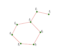
Dual Graph

The dual graph G associated to the mesh S is defined as follows:

• each vertex of G corresponds to a triangle of S,

• two vertices of G are neighbours (i.e., connected by an edge of the dual graph) if and only if their corresponding triangles in S share an edge.

Original Mesh

Dual Graph

Dual Graph Decimation
Once the dual graph G is computed, the algorithm starts the decimation stage which consists in successively applying halfe-edge collapse decimation operations. Each half- edge collapse operation applied to an edge (v,w), denoted hecol(v, w), merges the two vertices v and w. The vertex w is removed and all its incident edges are connected to v.

HACD implementation details
How to improve HACD?
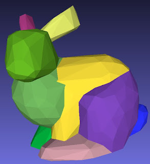
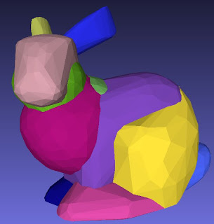
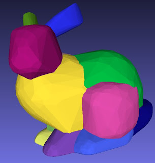
HACD parameter tweaking
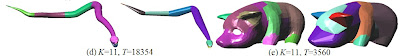
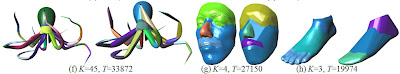
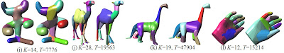
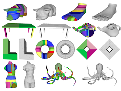
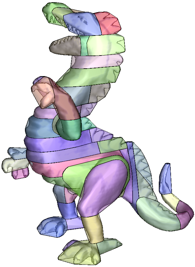
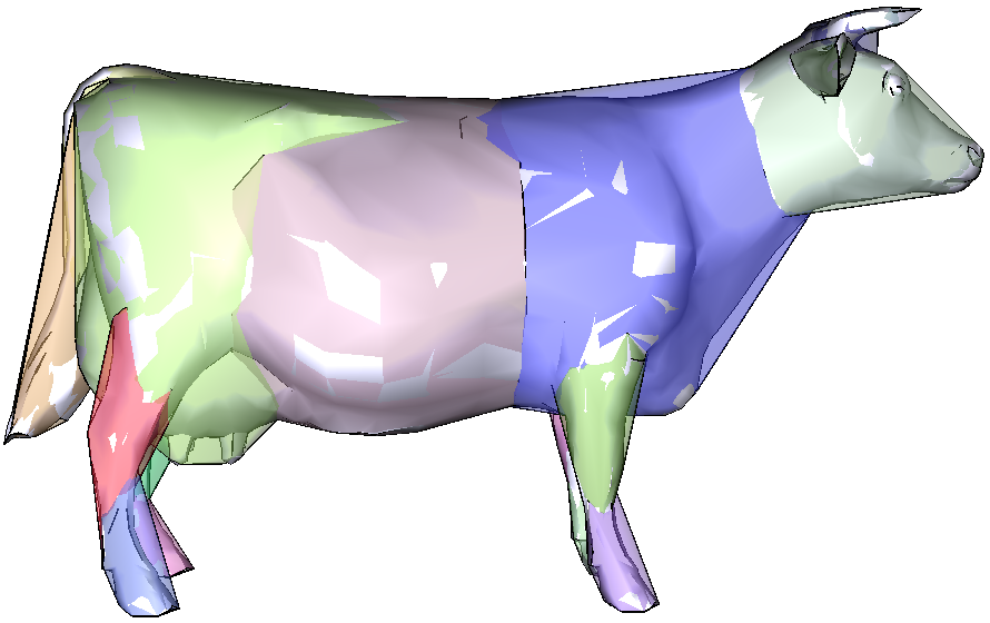
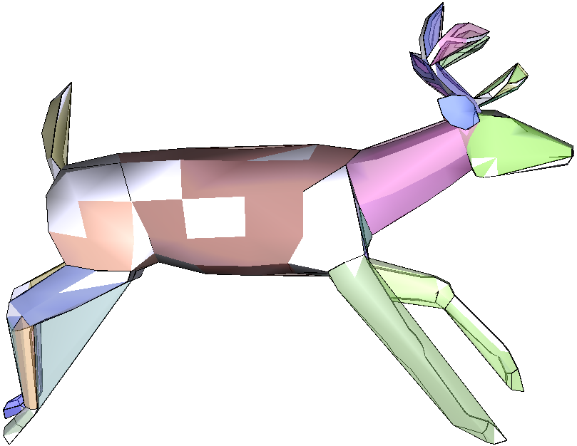
HACD decomposition results

HACD vs John Ratcliff's ACD library

---

HACD optimization

October 5, 2011, 6:56 am

≫ Next: HACD parameters

≪ Previous: HACD: Hierarchical Approximate Convex Decomposition

$

0

0

Today, I have updated the HACD library in order to reduce both memory usage and computation complexity (cf. http://sourceforge.net/projects/hacd/). 

The new version:

• uses John's Micro Allocator to avoid intensive dynamic memory allocation (thanks John for the great work),
• exploits a simplified version of  an axis-aligned-bounding-volume AABB tree to accelerate dual graph generation (the code is inspired by John's post on this subject, thanks again John :) )
• has an integrated mesh simplification pre-processing step, which makes it possible to handle dense meshes.

In this post, I'll give more details about this last feature.

To enable mesh decimation, the user specifies the target number of triangles that should be produced before running the convex decomposition. HACD will handle automatically the simplification and the decomposition processes. For the details of the mesh decimation algorithm, have a look at Michael Garland's  webpage http://mgarland.org/research/thesis.html. To turn this feature off just set the parameter targetNTrianglesDecimatedMesh=0.

I have tested the updated HACD algorithm on the 3D model "Bunny", which has 70K triangles. The HACD's parameters were set as follows:

• minNClusters = 12
• maxConcavity = 1000
• addExtraDistPoints = 1
• addFacesPoints = 1
• ConnectedComponentsDist = 30
• targetNTrianglesDecimatedMesh = 500, 1000, 2000, 4000, 8000 and 16000.

The snapshots of the produced convex decompositions are reported below. The computation times on my machine (Mac Intel Core 2 Duo, 4 GB RAM DDR3) ranged between 3 sec. for 500 triangles and 200 sec. for 16000 triangles (cf. Table 1 for the details).

----------------------------------------

# triangles Time (sec.)

----------------------------------------

5002.8

10004.6

200010

400021

800070

16000192

----------------------------------------

Table 1. Computation times for targetNTrianglesDecimatedMesh= 500, 1000, 2000, 4000, 8000 and 16000 

# triangles after simplification - 500

# triangles after simplification - 1000

# triangles after simplification - 2000

# triangles after simplification - 4000

# triangles after simplification - 8000

# triangles after simplification - 16000

HACD parameters

November 23, 2011, 2:51 pm

≫ Next: Article 20

≪ Previous: HACD optimization

$

0

0

In this post, I'll to give an overview of the HACD parameters and explain their meaning and how they should be set. The text will be improved over time. My main concern is to have things written down for reference...

1. Parameters overview

Parameter	Description	Default
NTargetTrianglesDecimatedMesh	Target number of triangles in the decimated mesh. The decimation stage was added mainly to decrease the computation costs for dense meshes (refer to Section 2.1).	1000
NVerticesPerCH	Maximum number of vertices in the generated convex-hulls.	100
ScaleFactor	Normalization factor used to ensure that the other parameters (e.g. concavity) are expressed w.r.t. a fixed size. Refer to Section 2.3 for details	1000
SmallClusterThreshold	Threshold on the clusters area (expressed as a percentage of the entire mesh area) under which the cluster is considered small and it is forced to be merged with other clusters at the price of a high concavity.	0.25
AddFacesPoints	If enabled an additional ray located at the center of each triangle pointing toward its normal is considered when computing the concavity of a non-flat cluster. The parameter was added to handle coarse meshes (i.e. with a low number of vertices)	ON
AddExtraDistPoitns	If enabled additional rays are considered to handle bowl-like shapes.	ON
NClusters	Minimum number of convex-hulls to be generated	1
Concavity	Maximum allowed concavity	100
ConnectDist	If the distance between two triangles, each belonging to a different connected components (CCs), is lower than the ConnectDist threshold an additional edge connecting them is added to the dual graph. This parameter was added to handle meshes with multiple CCs.	30
VolumeWeight	Weight controlling the contribution of the volume related cost to the global edgecollapse cost (refer to XXX for details).	0.0 (not used)
CompacityWeight	Weight controlling the contribution of the shape factor related cost to the global edgecollapse cost (refer to XXX for details).	0.0001
FlatRegionThreshold	Threshold expressed a percentage of ScaleFactor under which a cluster is considered flat.	1
ComputationWeight	Weight controlling the contribution of the computation related cost to the global edgecollapse cost (refer to XXX for details).	0.01

2. Detailed description

• NTargetTrianglesDecimatedMesh

In order to reduce the computations times for dense meshes, the HACD library makes it possible to decimate the original mesh before running the decomposition process. More details about the decimation algorithm are provided here http://kmamou.blogspot.com/2011/10/hacd-optimization.html

• NVerticesPerCH

this parameter was introduced in order to comply with the constraints that most physics engines put on the number of vertices/triangles per convex-hull (CH). If the function HACD::Compute() is called with the parameter fullCH=false, then the generated CHs will have a number of vertices lower than NVerticesPerCH.

In order to optimally choose the best vertices to keep in the final CH, the ICHull::Process(unsigned long nPointsCH) function implements a slightly different version of the Incremental Convex Hull algorithm (cf. demo code ). Here, at each step, the point with the highest volume increment  is chosen, until all points are processed or the CH has exactly NVerticesPerCH points.

The code looks like this:

        while (!vertices.GetData().m_tag && addedPoints < nPointsCH) // not processed

        {

            if (!FindMaxVolumePoint())

            {

                break;

            }                 

            vertices.GetData().m_tag = true;                     

            if (ProcessPoint())

            {

                addedPoints++;

                CleanUp(addedPoints);

                vertices.Next();

            }

        }

        // delete remaining points

        while (!vertices.GetData().m_tag)

        {

            vertices.Delete();

        }

• ScaleFactor

A normalization process is applied to the input mesh in order to ensure that the other parameters (e.g. concavity) are expressed w.r.t. a fixed size. This process is inverted before producing the final CHs.

The HACD::Compute() function follows the following main steps:

    bool HACD::Compute(boolfullCH, bool exportDistPoints)

    {

        if (m_targetNTrianglesDecimatedMesh > 0)

        {

           DecimateMesh(targetNTrianglesDecimatedMesh);

        }

        NormalizeData();

        CreateGraph();

        InitializeDualGraph();

        InitializePriorityQueue();

        Simplify();

        DenormalizeData();

        CreateFinalCH();

        returntrue;

    }

The HACD::NormalizeData() function centers the mesh and scale it so its coordinates are in the interval [-m_sacle, m_sclae]x[-m_sacle, m_sclae]x[-m_sacle, m_sclae]. The code proceeds as follows:

       void HACD::NormalizeData()

       {

              const Real invDiag = static_cast<Real>(2.0 * m_scale / m_diag);

              for (size_t v = 0; v < m_nPoints ; v++)

              {

                     m_points[v] = (m_points[v] - m_barycenter) * invDiag;

              }

       }

The HACD::DenormalizeData() function invert the normalization operated by HACD::NormalizeData():

       void HACD::DenormalizeData()

       {

              constReal diag = static_cast<Real>(m_diag / (2.0 * m_scale));

              for(size_t v = 0; v < m_nPoints ; v++)

              {

                     m_points[v] = m_points[v] * diag + m_barycenter;

              }

      }

• SmallClusterThreshold

Due to numerical stability issues (or maybe some bugs I haven't spotted yet :) ) the HACD algorithm may produce small clusters. In order to detect them and make sure they will be merged, the SmallClusterThreshold was introduced. A cluster is considered to be small if its area is smaller than SmallClusterThreshold% of the entire mesh area.

The condition2 in the HACD::Simplify() function forces small clusters to be merged (m_area is the area of the entire mesh):

void HACD::Simplify()

       {

              double areaThreshold = m_area * m_smallClusterThreshold / 100.0;

              while ( !m_pqueue.empty() )

              {

               currentEdge = m_pqueue.top();

               m_pqueue.pop();

               v1 = m_graph.m_edges[currentEdge.m_name].m_v1;

               v2 = m_graph.m_edges[currentEdge.m_name].m_v2;

               boolcondition1 = (m_graph.m_edges[currentEdge.m_name].m_concavity <  

                                  m_concavity) && (globalConcavity < m_concavity) && 

                                  (m_graph.GetNVertices() > m_nMinClusters) && 

                                  (m_graph.GetNEdges() > 0);

              bool condition2 = (m_graph.m_vertices[v1].m_surf < areaThreshold || 

                                 m_graph.m_vertices[v2].m_surf < areaThreshold);

              if(condition1 || condition2)

              {

                   m_graph.EdgeCollapse(v1, v2);

                   long idEdge;

                   for(size_t itE = 0; itE < m_graph.m_vertices[v1].m_edges.Size(); ++itE)

                   {

                      idEdge = m_graph.m_vertices[v1].m_edges[itE];

                      ComputeEdgeCost(idEdge);                                            

                   }                 

              }

       }

• AddFacesPoints and AddExtraDistPoitns

The parameter AddFacesPoints was introduced to improve the precision of the concavity computation for meshes with a low number of vertices. The idea is to add additional rays located each at the center  of a triangle and pointing to the same direction as its normal.

The Parameter AddExtraDistPoints was added to handle bowl-like shapes. As illustrated below, if only the rays located on the current cluster are considered when computing its concavity, you may end up with a big cluster corresponding to the external surface (which is convex) of the bowl containing a lot of small clusters located on the internal part (which is concave). 

Bad decomposition for bowl-like shapes if AddExtraDistPoints is not enabled

In order to avoid such a bad decomposition, the idea consists in introducing new rays that would constrain the propagation of the cluster corresponding to the external surface of the bowl by taking into account rays located on the concave part. More precisely, during the initialization stage, an additional ray (the yellow ray in the figure below) is associated with each triangle (colored in red). 

The additional ray, denoted R (the yellow arrow), is defined as follows. Let N be the normal (the blue arrow) to the current triangle T (colored in red) and X be the ray starting at the center of T and with direction (-N) (the dotted green arrow). The starting point of R, denoted P0 (the yellow point), is defined a the nearest intersection point of X and the mesh. Moreover, the normal of the surface at P0 should point to the same direction as X. R has the direction of the normal of the surface at the P0.

Additional ray (yellow) is associated with the red triangle when AddExtraDistPoints is activated

The code looks like this:

    void HACD::InitializeDualGraph()

    {

         for(unsignedlong f = 0; f < m_nTriangles; f++)

        {

            i = m_triangles[f].X();

            j = m_triangles[f].Y();

            k = m_triangles[f].Z();

            m_graph.m_vertices[f].m_distPoints.PushBack(DPoint(i, 0, false, false));

            m_graph.m_vertices[f].m_distPoints.PushBack(DPoint(j, 0, false, false));

            m_graph.m_vertices[f].m_distPoints.PushBack(DPoint(k, 0, false, false));

           

            u = m_points[j] - m_points[i];

            v = m_points[k] - m_points[i];

            w = m_points[k] - m_points[j];

            normal = u ^ v;

            m_normals[i] += normal;

            m_normals[j] += normal;

            m_normals[k] += normal;

            m_graph.m_vertices[f].m_surf = normal.GetNorm();

            m_area += m_graph.m_vertices[f].m_surf;

            normal.Normalize();

            if(m_addFacesPoints)

            {

                m_faceNormals[f] = normal;

                m_facePoints[f] = (m_points[i] + m_points[j] + m_points[k]) / 3.0;

            }

            if (m_addExtraDistPoints)   

            {

                Vec3<Real> seedPoint((m_points[i] + m_points[j] + m_points[k]) / 3.0);

                Vec3<Real> hitPoint;

                Vec3<Real> hitNormal;

                normal = -normal;

                if(rm.Raycast(seedPoint,normal,hitTriangle,dist, hitPoint, hitNormal))

                {

                     faceIndex = hitTriangle;

                }  

                if (faceIndex < m_nTriangles )

                {

                     m_extraDistPoints[f] = hitPoint;

                     m_extraDistNormals[f] = hitNormal;                

                     m_graph.m_vertices[f].m_distPoints.PushBack(DPoint(m_nPoints+f, 0, false, true));

              }

            }

        }

        for (size_t v = 0; v < m_nPoints; v++)

        {

              m_normals[v].Normalize();

        }

    }

• Concavity

This parameter specifies the maximum allowed concavity for each cluster. As discussed in http://kmamou.blogspot.com/2011/10/hacd-hierarchical-approximate-convex.html different concavity measures are considered for flat (i.e. 2D) surfaces and for non-flat surfaces.

• ConnectDist

In order to handle meshes with different connected components. The idea consists  in adding "virtual edges" between triangles belonging to different CCs. More precisely, if the distance between two triangles T1 and T2 belonging each to a different CC is lower than a threshold distConnect then an edge connecting T1 to T2 is added to the dual graph.

The code looks like this:

       void HACD::CreateGraph()

    {

        …

        if (m_ccConnectDist >= 0.0)

        {

            m_graph.ExtractCCs();

            if (m_graph.m_nCCs > 1)

            {

                std::vector< std::set<long> > cc2V;

                cc2V.resize(m_graph.m_nCCs);

                long cc;

                for(size_t t = 0; t < m_nTriangles; ++t)

                {

                    cc = m_graph.m_vertices[t].m_cc;

                    cc2V[cc].insert(m_triangles[t].X());

                    cc2V[cc].insert(m_triangles[t].Y());

                    cc2V[cc].insert(m_triangles[t].Z());

                }

               

                for(size_t cc1 = 0; cc1 < m_graph.m_nCCs; ++cc1)

                {

                    for(size_t cc2 = cc1+1; cc2 < m_graph.m_nCCs; ++cc2)

                    {

                        std::set<long>::const_iterator itV1(cc2V[cc1].begin()), itVEnd1(cc2V[cc1].end());

                        for(; itV1 != itVEnd1; ++itV1)

                        {

                                                double distC1C2 = std::numeric_limits<double>::max();

                            double dist;

                            t1 = -1;

                            t2 = -1;

                            std::set<long>::const_iterator itV2(cc2V[cc2].begin()), itVEnd2(cc2V[cc2].end());

                            for(; itV2 != itVEnd2; ++itV2)

                            {

                                dist = (m_points[*itV1] - m_points[*itV2]).GetNorm();

                                if (dist < distC1C2)

                                {

                                    distC1C2 = dist;

                                    t1 = *vertexToTriangles[*itV1].begin();

                                   

                                                              std::set<long>::const_iterator it2(vertexToTriangles[*itV2].begin()),

                                                                                                                 it2End(vertexToTriangles[*itV2].end());

                                                              t2 = -1;

                                                              for(; it2 != it2End; ++it2)

                                                              {

                                                                     if (*it2 != t1)

                                                                     {

                                                                           t2 = *it2;

                                                                           break;

                                                                     }

                                                              }

                                }

                            }

                            if (distC1C2 <= m_ccConnectDist && t1 >= 0 && t2 >= 0)

                            {

                                m_graph.AddEdge(t1, t2);                   

                            }

                        }

                    }

                }

            }

        }

    }

•  FlatRegionThreshold

When computing concavity we need to distinguish between flat surfaces and non-float surfaces. The measure of flatness considered in HACD is related to the ratio between the convex-hull volume and the area of its boundary. If this later ration is small compared to m_scale then the mesh is considered flat. Otherwise it is considered non-flat. The parameter FlatRegionThreshold is the threshold which separate flat region from non flat region. It is expressed as percentage of m_scale.

In practice, the final concavity is computed as weighted sum of the flat region concavity and the 3D concavity. The weight is a function of the flatness of the cluster.

The code is as follows:

void HACD::ComputeEdgeCost(size_t e)

{

…

double surfCH = ch->ComputeArea() / 2.0;

double volumeCH = ch->ComputeVolume();

double vol2Surf = volumeCH / surfCH;

double concavity_flat = sqrt(fabs(surfCH-surf));

doubleweightFlat = std::max(0.0, 1.0 - pow(- vol2Surf * 100.0 / (m_scale * m_flatRegionThreshold), 2.0));

concavity_flat *= weightFlat;

if(!ch->IsFlat())

{

   concavity = Concavity(*ch, distPoints);

}

concavity += concavity_flat;

…

}

Article 20

November 7, 2012, 10:16 pm

≫ Next: Article 19

≪ Previous: HACD parameters

$

0

0

This post is out-of-date. Check out V-HACD 2.0!

V-HACD: Hierarchical Approximate Convex Decomposition Revisited

Lately, I have found time to work on improving the HACD algorithm. The new V-HACD library tries to tackle the problem of convex-hulls inter-penetration usually encountered when using HACD. Figure 1 illustrates this limitation by comparing V-HACD results to those generated by using HACD.

Figure 1. V-HACD vs. HACD: V-HACD generates non-overlapping convex-hulls.

V-HACD works only with manifold closed meshes of arbitrary genus, which makes it less general than HACD algorithm (which handles open and non-manifold meshes). The V-HACD code  is available under New BSD License. However, the current version relies on the following other libraries:

• Triangle to compute constrained delaunay triangulation which has a non permissive license, which should be replaced [Thanks to Erwin Coumans for noticing that]
• Ole Kniemeyer's implementation of the convex-hull algorithm provided with bullet
• John Tsiombikas's kd-tree algorithm

The first results are encouraging. However, the code is still buggy and not optimized. I hope that people would be interested in helping me improve this first version.

To play with the algorithm, a pre-compiled win32 executable is available here
Pre-computed decomposition results are available here

V-HACD parameters are the following:

testVHACD fileName.off depth maxConcavity invertInputFaces posSampling angleSampling posRefine angleRefine alpha targetNTrianglesDecimatedMesh

• fileName.off: 3D mesh in off format (type: string, example: block.off )
• depth: maximum number of decomposition stages (type: integer, default: 10)
• maxConcavity: maximum allowed concavity (type: float, default 0.01)
• invertInputFaces: indicates whether mesh normals should be inverted or not (type: boolean, default 0)
• posSampling: clipping plane position sampling resolution for coarse search (type: int, default 10)
• angleSampling: clipping plane orientation sampling resolution for coarse search (type: int, default 10) 
• posRefine: clipping plane position sampling resolution for refined search (type: int, default 5) 
• angleRefine: clipping plane orientation sampling resolution for refined search (type: int, default 5)
• alpha: parameter controlling the compromise between concavity and balance between convex-hulls. (type: float, default: 0.01)
• targetNTrianglesDecimatedMesh: number of triangles in the decimated mesh. V-HACD decimates the input mesh to reduce computation times. (type: integer, default: 1000)

To apply V-HACD to the input mesh "input.off" use the following command line:

testVHACD.exe input.off 30 0.01 0 64 32 8 64 0.001 2000

Below, some screen-shots of the obtained results.

The current version of V-HACD provides poor results or errors for the following three meshes. As soon as I get some free time I'll try to fix these bugs.

• dancer2
• elk
• hand1
• hand2
• hero
• octopus
• polygirl
• shark_b
• Sketched-Brunnen
• torus
• tstTorusModel
• tstTorusModel3

Article 19

November 12, 2012, 6:56 pm

≫ Next: Open3DGC (Open 3D Graphics Compression)

≪ Previous: Article 20

$

0

0

V-HACD: Replacing Triangle's Constrained Delaunay Triangulation

As mentioned in my previous post, the first version of V-HACD relies on the library Triangle to compute 2D constrained Delaunay triangulations. In fact, the V-HACD algorithm involves clipping the mesh against a plane and filling the produced holes (cf. Figure 1).

The Triangle library produces excellent results and is very stable. However, as pointed out by Erwin Coumans it has a non permissive license. Another alternative to Triangle is the poly2tri, which is released under a New BSD License. Poly2tri turned out to be non-usable in my case because it supports only simple polygons as constraints. After searching the internet for a "good" and stable implementation with a permissive license, I ended up developing a simple triangulation algorithm (it is not a Constrained Delaunay Triangulation), which is enough for V-HACD needs. My implementation is a very simplified version of the Incremental Delaunay algorithm 

The new triangulation algorithm was uploaded to the git repository and could be compared to the Triangle library by adding #define USE_TRIANGLE to vhacdMesh.cpp

The code is still ugly and not optimized at all. For now, I am trying to have some first results and understand better the algorithm limitations. Hopefully, I'll have soon the time to clean up the code.

Open3DGC (Open 3D Graphics Compression)

July 24, 2013, 5:07 pm

≫ Next: Open3DGC at "COLLADA/glTF" BoF (Siggraph 2013)

≪ Previous: Article 19

$

0

0

I am glad to introduce the Open3DGC (Open 3D Graphics Compression) library!

Open3DGC aims at providing a cross platform C++ implementation (under MIT License) of patent free MPEG tools for 3D graphics compression.

The current Open3DGC version provides an implementation of the MPEG-SC3DMC codec  (Scalable Complexity 3D Mesh Compression). SC3DMC  offers an efficient low complexity solution to compress arbitrary triangular 3D meshes with attributes (e.g., normals, texture coordinate, skinning animation weights, bone IDs..).

A detailed description of the compression algorithm is available here

Open3DGC supports two output stream types:

• Binary streams: compressed using arithmetic encoding
• ASCII (7-bits) streams: adapted for server-side gzip compression and java-script client side decoding

Compression Efficiency

Open3DGC is 7.8 times more efficient than Gzip and 

1.7-2.0 times more efficient than Webgl-loader and OpenCTM

• Test dataset: 160 models with various shapes and topologies (i.e., open/closed, manifold/non-manifold, arbitrary genus)
• Codecs: 
• WebGL-Loader  and Open3DGC with 14 bits quantization for positions and 10 bits quantization for normals/texture coord
• OpenCTM: default parameters  (not fair)

Using the Open3DGC Compression Tool

• The "test_o3dgc" tool supports only OBJ files with a single triangular model
• Pre-built binaries for Win32, Win64 and ubuntu are available here
• Example of test models are located here
• To compress the "bunny" model file use the following command line:

• Binary stream

test_o3dgc.exe -c -st binary -i bunny.obj

• ASCII stream

test_o3dgc.exe -c -st ascii -i bunny.obj

• ASCII streams should be further compressed by using GZip

• To decompress the stream:

test_o3dgc.exe -d -i bunny.s3d

• 
  

Open3DGC at "COLLADA/glTF" BoF (Siggraph 2013)

July 27, 2013, 10:06 pm

≫ Next: Open3DGC (updated results)

≪ Previous: Open3DGC (Open 3D Graphics Compression)

$

0

0

Open3DGC was demoed at "COLLADA/glTF" BoF (Siggraph 2013). Check out these two presentations:

• Graphics Library Transmission Format (Fabrice Robinet)
• Rest3D (Remi Arnaud)

Open3DGC (updated results)

July 31, 2013, 10:37 pm

≫ Next: Open3DGC (more results!)

≪ Previous: Open3DGC at "COLLADA/glTF" BoF (Siggraph 2013)

$

0

0

In a previous post, I reported experimental results comparing the compression efficiency of Open3DGCto webgl-loader and OpenCTM. In this post, I am providing an updated version, which takes into account:

• The "evaluation version"obj2utf8x of webgl-loader, which provides better compression performances than the obj2utf8 encoder, and
• The latest Open3DGC version (slightly better compression).

  

---

Open3DGC (more results!)

August 1, 2013, 5:47 pm

≫ Next: [Open3DGC] Examples of encoded streams

≪ Previous: Open3DGC (updated results)

$

0

0

Encoders

• Open3DGC-Bin: binary version of Open3DGC (14 bits quantization)
• Open3DGC-ASCII: ascii version of Open3DGC (14 bits quantization)
• webgl-loader: the optimized version obj2utf8x (14 bits quantization)
• GZip (default): level=6
• GZip (best): level=9
• 7zip (best): level=9

Test dataset

Results

[Open3DGC] Examples of encoded streams

August 1, 2013, 9:59 pm

≫ Next: Selecting O3DGC Encoding Parameters

≪ Previous: Open3DGC (more results!)

$

0

0

Encoded Models

• Bunny
• Buddha
• Ben
• Dragon

Original, encoded and decoded streams are available here 

Compression Results

• 14 bits quantization for positions
• 10 bits quantization for normals and texture coordinates

Selecting O3DGC Encoding Parameters

October 8, 2013, 8:23 pm

≫ Next: AMD VIDEO CODING ENGINE: THE ROUTE TOWARDS LOW-LATENCY CLOUD GAMING SOLUTIONS

≪ Previous: [Open3DGC] Examples of encoded streams

$

0

0

Attribute type	Quantization	Prediction mode
POSITION	Excellent quality: 13 Good quality: 12 Aggressive compression: 10	O3DGC_SC3DMC_PARALLELOGRAM_PREDICTION
TEXCOORD	10 (for 1024x1024) texture images 9 (for 512x512) texture images 8 (for 256x256) texture images N (for 2^Nx2^N) texture images	O3DGC_SC3DMC_PARALLELOGRAM_PREDICTION
NORMAL	Excellent quality: 10 Good quality: 8 Aggressive compression: 6	O3DGC_SC3DMC_SURF_NORMALS_PREDICTION if the normals magnitudes are not relevant O3DGC_SC3DMC_PARALLELOGRAM_PREDICTION to preserve the normals magnitudes
COLOR	Excellent quality: 10 Good quality: 8 Aggressive compression: 6	O3DGC_SC3DMC_DIFFERENTIAL_PREDICTION
WEIGHT	No idea yet. I need to test with real data. I would say between 8-12	O3DGC_SC3DMC_PARALLELOGRAM_PREDICTION
JOINT_ID	No quantization	O3DGC_SC3DMC_DIFFERENTIAL_PREDICTION

Computational complexity of prediction modes:

·         O3DGC_SC3DMC_PARALLELOGRAM_PREDICTION (+++)

·         O3DGC_SC3DMC_SURF_NORMALS_PREDICTION (+++)

·         O3DGC_SC3DMC_DIFFERENTIAL_PREDICTION (++)

·         O3DGC_SC3DMC_NO_PREDICTION (+)

AMD VIDEO CODING ENGINE: THE ROUTE TOWARDS LOW-LATENCY CLOUD GAMING SOLUTIONS

November 23, 2013, 3:38 pm

≫ Next: EFFICIENT 3D WEB CONTENT DELIVERY WITH KHRONOS AND MPEG TECHNOLOGIES

≪ Previous: Selecting O3DGC Encoding Parameters

$

0

0

EFFICIENT 3D WEB CONTENT DELIVERY WITH KHRONOS AND MPEG TECHNOLOGIES

November 23, 2013, 3:42 pm

≫ Next: V-HACD V2.0 is here!

≪ Previous: AMD VIDEO CODING ENGINE: THE ROUTE TOWARDS LOW-LATENCY CLOUD GAMING SOLUTIONS

$

0

0

glTF Viewer leveraging Open3DGC compression

V-HACD V2.0 is here!

November 11, 2014, 11:15 pm

≫ Next: Using the V-HACD library in your project

≪ Previous: EFFICIENT 3D WEB CONTENT DELIVERY WITH KHRONOS AND MPEG TECHNOLOGIES

$

0

0

V-HACD V2.0 is here and it kicks ass. It works with any triangular mesh (i.e., open or closed, manifold or not, oriented or not...) and it gives cleaner and more consistent results than V-HACD 1.0 and HACD.

The source code is available here https://code.google.com/p/v-hacd/

You can also download binaries:

• win32
• win64
• ubuntu
• osx

Example of command line (lower quality but faster):

testVHACD.exe input.obj 100000 20 0.0025 4 4 0.05 0.05 0.00125 0 0 64 0.0 output.wrl log.txt

Example of command line (high quality but slow):

testVHACD.exe input.obj 8000000 20 0.0025 4 4 0.05 0.05 0.00125 0 0 64 0.0 output.wrl log.txt

Below some convex decomposition results generated with V-HACD 2.0.

Using the V-HACD library in your project

December 6, 2014, 5:38 am

≫ Next: V-HACD 2.0 vs. HACD

≪ Previous: V-HACD V2.0 is here!

$

0

0

I have lately worked on re-factoring the V-HACD code to make it easier to integrate. An example of code using V-HACD would look like this.

1 2 3 4 5 6 7 8 9 10 11 12 13 14 15 16 17 18 19 20 21 22 23 24 25 26 27 28 29 30 31 32 33 34 35 36

#include <stdio.h> #include "VHACD.h" intmain(int argc, char* argv[]) { int* triangles; // array of indexes float* points; // array of coordinates ... // load the mesh ... IVHACD::Parameters params; // V-HACD parameters IVHACD * interfaceVHACD = CreateVHACD(); // create interface // compute approximate convex decomposition bool res = interfaceVHACD->Compute(points, 3, nPoints, triangles, 3, nTriangles, params); // read results unsignedint nConvexHulls = interfaceVHACD->GetNConvexHulls(); // Get the number of convex-hulls IVHACD::ConvexHull ch; for (unsignedint p =0; p < nConvexHulls; ++p) { interfaceVHACD->GetConvexHull(p, ch); // get the p-th convex-hull information for (unsignedint v =0, idx =0; v < ch.m_nPoints; ++v, idx+=3) { printf("x=%f, y=%f, z=%f", ch.m_points[idx], ch.m_points[idx+1], ch.m_points[idx+2]) } for (unsignedint t =0, idx =0; t < ch.m_nTriangles; ++t, idx +=3) { printf("i=%f, j=%f, k=%f", ch.m_triangles[idx], ch.m_triangles[idx+1], ch.m_triangles[idx+2]) } } // release memory interfaceVHACD->Clean(); interfaceVHACD->Release(); return0; }

All the magic happens at line 14 where the IVHACD::Compute() function is called. In order to cancel the decomposition process, the function IVHACD::Cancel() could be called from any other thread.

V-HACD offers the user the possibility to track progress and get access to logging information. The only thing the user needs to do is to provide his implementation of the two abstract classes IUserCallback and IUserLogger.

Below, an example of implementation of IUserCallback.

1 2 3 4 5 6 7 8 9 10 11 12 13 14 15 16

classMyCallback:public IVHACD::IUserCallback { public: MyCallback(void) {} ~MyCallback() {}; voidUpdate(constdouble overallProgress, constdouble stageProgress, constdouble operationProgress, constchar*const stage, constchar*const operation) { cout << setfill('') << setw(3) << (int)(overallProgress +0.5) <<"% " <<"[ "<< stage <<""<< setfill('') << setw(3) << (int)(stageProgress +0.5) <<"% ] " << operation <<""<< setfill('') << setw(3) << (int)(operationProgress+0.5) <<"%"<< endl; }; };

The Update() callback is called regularly during the decomposition process to report:

• The overall progress,
• The progress of the current stage, and
• The progress of the current operation.

Notice that the progress is always reported as a percentage. The decomposition process is composed of a set of stages, which are composed of operations.

An example of implementation of IUserLogger may look as follows.

1 2 3 4 5 6 7 8 9 10 11 12 13 14 15 16 17 18

classMyLogger:public IVHACD::IUserLogger { public: MyLogger(void){} MyLogger(const string & fileName){ OpenFile(fileName); } ~MyLogger() {}; voidLog(constchar*const msg) { if (m_file.is_open()) { m_file << msg; m_file.flush(); } }; voidOpenFile(const string & fileName) { m_file.open(fileName.c_str()); } private: ofstream m_file; };

MyCallback and MyLogger are hooked to the IVHACD object by updating encode parameters as follows.

1 2 3 4 5 6 7 8 9 10

IVHACD::Parameters params; // V-HACD parameters IVHACD * interfaceVHACD = CreateVHACD(); // create interface MyCallback myCallback; MyLogger myLogger(fileNameLog); params.m_logger =&myLogger; params.m_callback =&myCallback; // compute approximate convex decomposition bool res = interfaceVHACD->Compute(points, 3, nPoints, triangles, 3, nTriangles, params);

---

V-HACD 2.0 vs. HACD

December 7, 2014, 6:46 pm

≫ Next: V-HACD 2.0 Parameters Description

≪ Previous: Using the V-HACD library in your project

$

0

0

Below some approximate convex decomposition results comparing V-HACD 2.0 and HACD.

Parameters:

• testVHACD.exe %%i 8000000 20 0.003 4 4 0.05 0.05 0.0015 0 0 256 0.0 %%i.wrl log_%%i.txt
• testHACD.exe %%i  2 50 0 0 1 30 2000

Score:

• +1: V-HACD provides better decomposition than HACD
• -1: HACD provides better decomposition than V-HACD
• 0: V-HACD and HACD provide comparable results

V-HACD 2.0	HACD	Score
18 convex-hulls	66 convex-hulls	1
18 convex-hulls	26 convex-hulls	1
16 convex-hulls	12 convex-hulls	-1
30 convex-hulls	28 convex-hulls	0
46 convex-hulls	54 convex-hulls	1
18 convex-hulls	26 convex-hulls	1
16 convex-hulls	19 convex-hulls	0
18 convex-hulls	22 convex-hulls	0
34 convex-hulls	17 convex-hulls	1
18 convex-hulls	13 convex-hulls	-1
25 convex-hulls	28 convex-hulls	1
20 convex-hulls	15 convex-hulls	-1
22 convex-hulls	16 convex-hulls	-1
42 convex-hulls	42 convex-hulls	0
9 convex-hulls	7 convex-hulls	-1
16 convex-hulls	15 convex-hulls	1
35 convex-hulls	37 convex-hulls	0
17 convex-hulls	17 convex-hulls	0
18 convex-hulls	18 convex-hulls	0
36 convex-hulls	34 convex-hulls	0
13 convex-hulls	10 convex-hulls	-1
11 convex-hulls	5 convex-hulls	-1
24 convex-hulls	20 convex-hulls	1
35 convex-hulls	36 convex-hulls	0
21 convex-hulls	13 convex-hulls	-1
15 convex-hulls	16 convex-hulls	0
9 convex-hulls	10 convex-hulls	0
41 convex-hulls	71 convex-hulls	0
22 convex-hulls	27 convex-hulls	0
47 convex-hulls	51 convex-hulls	0
23 convex-hulls	28 convex-hulls	0

V-HACD 2.0 Parameters Description

December 13, 2014, 2:32 pm

≫ Next: V-HACD Blender Add-on (by Alain Ducharme)

≪ Previous: V-HACD 2.0 vs. HACD

$

0

0

Parameter name	Description	Default value	Range
resolution	maximum number of voxels generated during the voxelization stage	100,000	10,000-64,000,000
depth	maximum number of clipping stages. During each split stage, all the model parts (with a concavity higher than the user defined threshold) are clipped according the "best" clipping plane	20	1-32
concavity	maximum concavity	0.0025	0.0-1.0
planeDownsampling	controls the granularity of the search for the "best" clipping plane	4	1-16
convexhullDownsampling	controls the precision of the convex-hull generation process during the clipping plane selection stage	4	1-16
alpha	controls the bias toward clipping along symmetry planes	0.05	0.0-1.0
beta	controls the bias toward clipping along revolution axes	0.05	0.0-1.0
gamma	maximum allowed concavity during the merge stage	0.00125	0.0-1.0
pca	enable/disable normalizing the mesh before applying the convex decomposition	0	0-1
mode	0: voxel-based approximate convex decomposition, 1: tetrahedron-based approximate convex decomposition	0	0-1
maxNumVerticesPerCH	controls the maximum number of triangles per convex-hull	64	4-1024
minVolumePerCH	controls the adaptive sampling of the generated convex-hulls	0.0001	0.0-0.01

V-HACD Blender Add-on (by Alain Ducharme)

December 15, 2014, 10:15 am

≫ Next: Who is using V-HACD?

≪ Previous: V-HACD 2.0 Parameters Description

$

0

0

Checkout this Blender add-on released by Alain Ducharme!

Who is using V-HACD?

December 16, 2014, 9:21 pm

≫ Next: [V-HACD] Adaptive Convex-Hulls Sub-sampling

≪ Previous: V-HACD Blender Add-on (by Alain Ducharme)

$

0

0

Please, let me know if you are using V-HACD in your products

• Leadwerks
• 3DEXCITE
• Unreal Engine 4
• DBPro
• HighFidelity
• Bonzai Engine

[V-HACD] Adaptive Convex-Hulls Sub-sampling

December 18, 2014, 6:48 pm

≫ Next: OpenCL Acceleration for V-HACD

≪ Previous: Who is using V-HACD?

$

0

0

Today, I took some time to add a new parameter (i.e., minVolumePerCH) to V-HACD to adaptively control the number of vertices/triangles of the generated convex-hulls. Below some results for different values of minVolumePerCH.